File IO

Examples

Download Sample Files

Read CSV Example

• read_csv-v1.py

• GHCN_sample.csv

Read/Write CSV Example

• rw_csv-v2.py

• GHCN_sample.csv

Read NetCDF Example

• read_netcdf-v2.py

• oisst_monthly.nc

• lsmask.nc

Read multiple NetCDF Example

• read-multi_netcdf-v2.py

• hgt_ncep_daily.2018.nc

• hgt_ncep_daily.2019.nc

• hgt_ncep_daily.2020.nc

Read/Write NetCDF Example

• rw_netcdf-v2.py

• oisst_monthly.nc

• lsmask.nc

CSV file

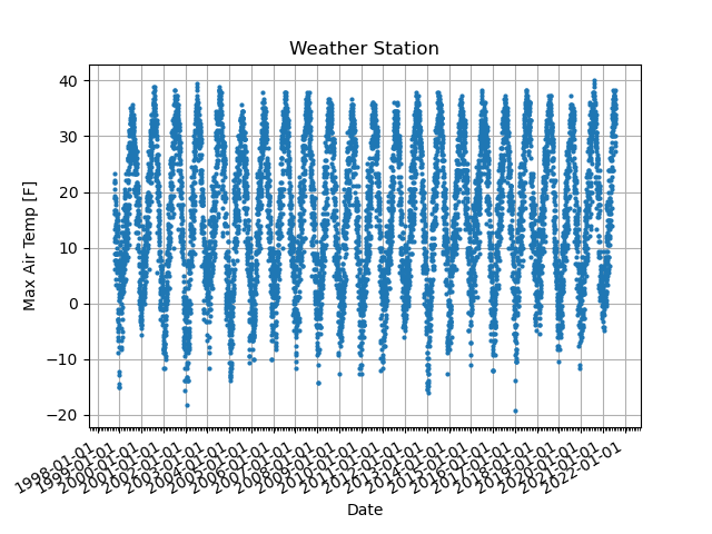
The CSV file is the typical format for weather station data. It stands for the “comma separated value” written by the text (or ASCII) format. It generally consists of data description (called a header) and data value. The package Pandas provides an easy way to read CSV files.

An example of CSV file

Let’s try to read the CSV file GHCN_sample.csv. This CSV file includes a note on Lines 1-15 and a header on Line 16. After Line 17, we can see the data separated by a comma. The value “M” indicates a missing value. The data contains day, precipitation, multi-day precipitation, snow depth, snowfall, minimum temperature, maximum temperature, and reference evapotranspiration.

This data has been provided by the Utah Climate Center. Please cite the Climate Center when using this data.
Station Network,GHCN:AWOS
Station ID,USW00094128
Station Name,LOGAN CACHE AP
Latitude,41.7872
Longitude,-111.8533
Elevation,1357.6 m
State,UT
Country,US
Units,Metric
*Note: 'S' Indicates a row that has been filled in by the system as a missing day.
*Note: All data is displayed the same as we receive it. If there are any values that may seem wrong
then download the data again and select the 'Show source/quality' option to view the flags.


Day,Precipitation,Multi-Day Precipitation,Snow Depth,Snow Fall,Min Temperature,Max Temperature,Ref Evapotranspiration
1998-10-01,M,M,M,M,M,M,M
1998-10-02,M,M,M,M,M,M,M
1998-10-03,M,M,M,M,M,M,M
1998-10-04,4.3,M,M,M,0.6,8.9,1.48056

An example of Python script

Let’s check the sample file, rw_csv-v2.py, to read and write a CSV file.

General packages

import numpy as np
import pandas as pd
import xarray as xr
import os
import matplotlib.pyplot as plt
import matplotlib.dates as mdates
from datetime import datetime

This script will read the CSV file using Pandas and then get the data as Xarray (and Numpy). There are some date formats in weather station data. For example, we describe August 24, 2021, as of 10-21-2021 or 10/21/21. The “DateTime” package is convenient to adjust such a date format. The “OS” package is also helpful to obtain the filename. This script also displays a plot using the package “Matplotlib,” but it is optional here.

Read a CSV file

# ----- Parameter setting ------
# == Date ==
dateparse = lambda x: datetime.strptime(x, '%Y-%m-%d')
#dateparse = lambda x: datetime.strptime(x, '%Y-%m-%d %H:%M:%S')
#dateparse = lambda x: datetime.strptime(x, '%m/%d/%y %H:%M')

# == CSV file name and location"
fcsv = 'GHCN_sample.csv'

# == Your definition of variable names
## Day,Precipitation, Multi-Day Precipitation, Snow Depth, Snow Fall, Min Temperature, Max Temperature, Ref Evapotranspiration,
vnames = ['date','precip','mdpr','sdep','sfall','tmin','tmax','refe']  

# == location of header. It starts from 0
nhead = 13

# == Figure name ==
fnFIG = os.path.splitext(os.path.basename(__file__))[0]

# ------------------------------

print(' ----- Read CSV file ------')
# additional parameters: encoding = 'ISO-8859-1'
fin = pd.read_csv(fcsv, \
	 delimiter = ',', header = nhead,  na_values = ['M','T','S'],\
         names = vnames, parse_dates = ['date'], date_parser = dateparse)


print(fin)
print(' ----------------------------')

print(' ----- Time setting ------')
date = fin.date.astype('datetime64[D]')
print(date)
print(' ----------------------------')

print(' ----- Get Maximum Temperature ------')
tmax = xr.DataArray(fin.tmax.astype(float), dims=('date'), coords={'date': date})
tmin = xr.DataArray(fin.tmin.astype(float), dims=('date'), coords={'date': date})

This script uses “pandas.read_csv” function to read the CSV file (Line 33-35). There are some options in this function. The option delimiter should be “,” for the CSV file. This script defines the file name (Line 17), the number of lines for the header (Line 24), and the missing value (na_values). It also defines the variable names on Line 21. The variable name in the first column is “date” here. The CSV file shows the date formate of October 1, 1998, as “1998-10-01”. Here, we define the date formate as “%Y-%m-%d” on Line 12, which puts into the option of “parse_dates” and “date_parser” for the function.

Note

Here are examples of date format.

• %Y-%m-%d (e.g., 2021-10-13)

• %m/%d/%y (e.g., 10/13/21)

• %Y-%d-%m %H:%M:%S (e.g., 2021-10-13 00:00:00)

Write a CSV file

df = pd.DataFrame ({'date': date, 'tavg': tavg, 'tmin': tmin, 'tmax': tmax})
df.to_csv(fnFIG+".csv",index=False)
print(df)

To write a CSV file, we use a Pandas function pandas.DataFrame.to_csv. An output file name has the same file name of this script as defined on Line 27, but for the CSV file extension (“.csv”). The output CSV file looks like below.

date,tavg,tmin,tmax
1998-10-01,,,
1998-10-02,,,
1998-10-03,,,
1998-10-04,4.75,0.6,8.9

NetCDF file

Read and write a single NetCDF file

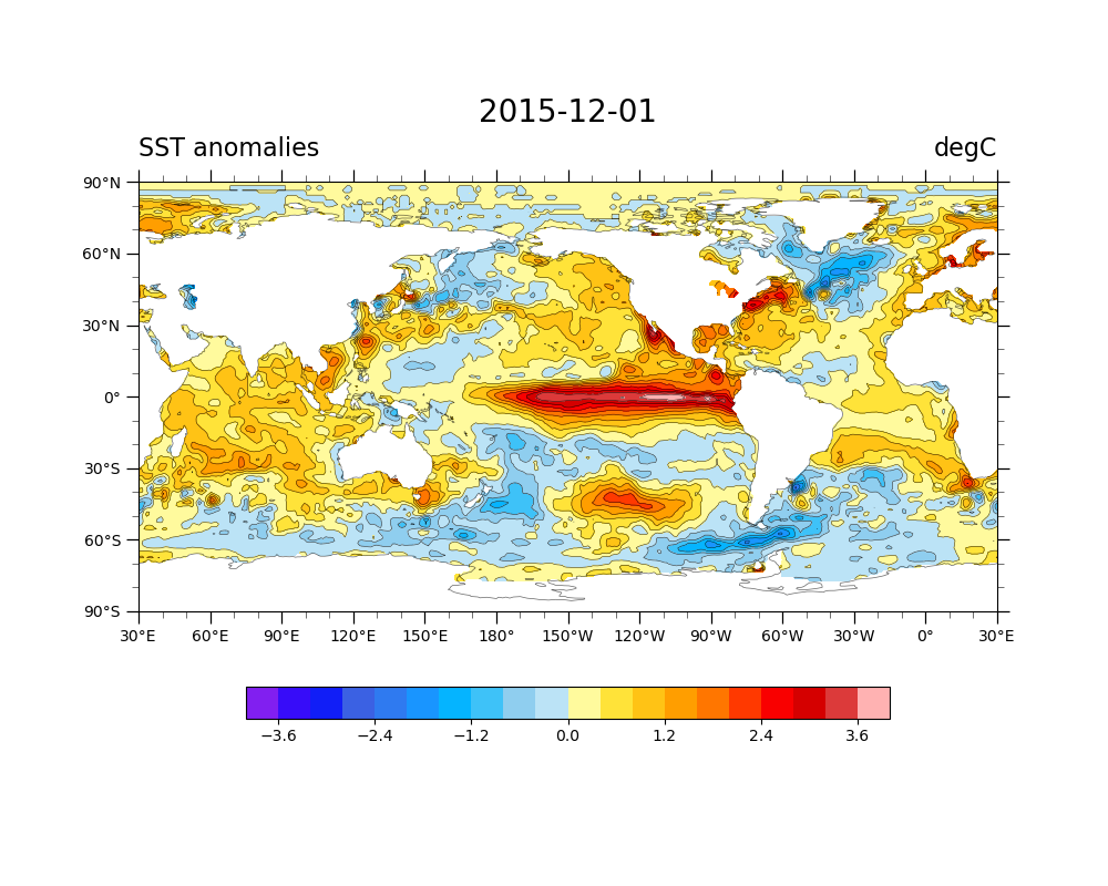
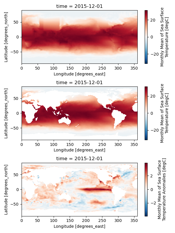
Let’s check the sample file, rw_netcdf-v2.py, to read and write a NetCDF file. This script reads monthly sea surface temperature provided by NOAA (oisst_monthly.nc). It also requires the land-sea mask file (lsmask.nc).

General packages

import numpy as np
import pandas as pd
import xarray as xr
import matplotlib.pyplot as plt
import matplotlib.dates as mdates
from datetime import datetime

This script uses Xarray to read and write the NetCDF file. As a default setting, Xarray may not support the NetCDF. In that case, you need to install other packages, such as Dask, NetCDF4, or PyNIO. Please check Install Packages how to install NetCDF.

Read a NetCDF file

# ----- Parameter setting ------

# == Figure name ==
fnFIG = 'rw_netcdf-v2.png'

sdate = '1982-01-01'
edate = '2020-12-01'

# -- Draw date
ddate = '2015-12-01'

# == netcdf file name and location"
fnc = 'oisst_monthly.nc'
dmask = xr.open_dataset('lsmask.nc')
print(dmask)


# == read netcdf data 
ds = xr.open_dataset(fnc)
print(ds)

sst = ds.sst.where(dmask.mask.isel(time=0) == 1)

clm = sst.sel(time=slice(sdate,edate)).groupby('time.month').mean(dim='time')
anm = (sst.groupby('time.month') - clm)
#print(clm)
#print(anm)

To read a signle NetCDF file, we use a xarray function xarray.open_dataset, as described on Lines 21 and 26. The resultant varialbe “ds” is the DataSet array. You can extract the sea surface temperature DataArray from “ds” on Line 29. We also applied the land-sea mask to obain the sea surface temperature over the ocean not the land using a DataArray.where function.

Read multiple NetCDF files

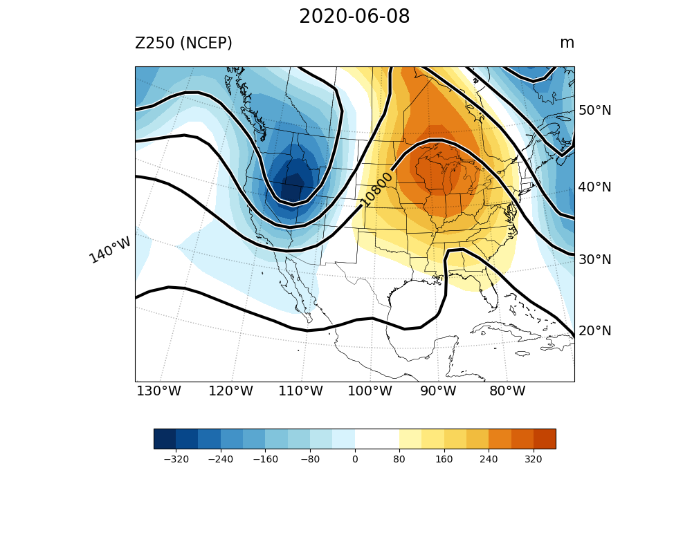
To read multiple NetCDF file, we use the differnet xarray function xarray.open_mfdataset. Following is an example to read the mulple NetCDF file and extract geopotential height at 250 hPa as the DataArray “dat”.

Sample file read-multi_netcdf-v2.py

# == netcdf file name and location"
fnc = "hgt_ncep_daily.*.nc"

ds = xr.open_mfdataset(fnc,  parallel=True)
print(ds)

dat = ds.hgt.sel(level=250)
print(dat)