1.1 Course Overview
Learning Objectives
After completing this lecture, students should be able to:
- Describe the goals and structure of this course.
- Explain how climate modeling integrates scientific knowledge, mathematics, and computational methods.
- Identify different types of climate models and recognize examples of climate model simulations.
- Prepare the Python environment required for the course.
Concept
The goal of this course is to demonstrate the integration of three essential components of climate modeling:
- scientific knowledge
- mathematics
- computational techniques
Climate models are built by combining these elements. Scientific understanding provides the physical processes that govern the climate system. Mathematics expresses these processes as equations. Computational methods then allow us to solve these equations numerically.
In other words, climate modeling requires the integration of science, mathematics, and computing.
This course is designed to help students develop these integrated skills by implementing simplified numerical models and performing computational experiments using Python.
Types of Climate Models
Climate models can take many forms depending on the level of complexity and the scientific questions being addressed. In general, climate models can be categorized into several types:
- Conceptual models
- Statistical models
- General circulation models (GCMs)
- Fully coupled Earth system models (ESMs)
Conceptual models use simplified equations to represent key physical mechanisms in the climate system. These models help us understand the fundamental dynamics of climate variability.
Statistical models use relationships derived from observational data to describe and predict climate behavior.
General circulation models simulate the large-scale circulation of the atmosphere and ocean using numerical solutions of physical equations.
Earth system models extend general circulation models by including additional components such as the carbon cycle, land processes, and biogeochemical interactions.
In this course, we will focus primarily on simplified conceptual models that illustrate important physical processes. These models allow us to clearly understand how mathematical equations and computational methods are used to simulate climate dynamics.
Examples that we will explore during the course include:
- a sine curve representing the seasonal cycle
- tendency equations describing time evolution
- advection and diffusion processes
- the Lorenz model illustrating chaotic behavior
The simplified models used in this course follow a workflow that is conceptually similar to the structure of more complex climate models such as general circulation models (GCMs) and Earth system models (ESMs).
Although the models we implement are much simpler, they share several important features commonly used in large-scale climate modeling systems:
- numerical integration of time-evolution equations
- use of model parameters and external forcing
- execution of simulations through scripts
- analysis and visualization of model output
By working with these simplified models, students can efficiently learn how numerical climate experiments are designed, executed, and interpreted. This approach provides a practical foundation for understanding more complex climate modeling frameworks used in research.
Sample Simulations
To illustrate what climate models can simulate, we will examine several example simulations.
These examples demonstrate how numerical models are used to represent complex climate processes and predict future climate behavior.
Examples shown in this lecture include:
-
High-resolution Earth simulation (YouTube)
-
KAKUSHIN Project simulation
-
Example simulations developed in this course
Later in the course we will reproduce simplified versions of climate processes using numerical models, including:
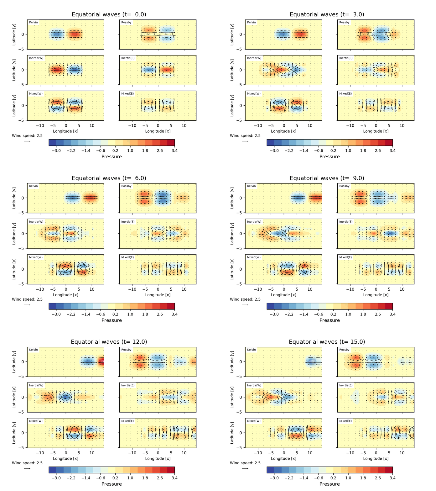
These examples illustrate how simplified models can capture important aspects of climate dynamics and help us understand the behavior of more complex climate models.
Exercise
- Install a terminal application if it is not already available on your computer.
- Install Miniconda.
- Create the course environment
env_psc6125. - Activate the environment.
- Verify that the required Python packages and FFmpeg are installed successfully.
Terminal and Miniconda installation instructions are available in the course GitHub repository:
Climate Data Analysis Setup Guide
Create the course environment
For most computers, we recommend using Python 3.12. If you are using an older computer or a Linux server with an older operating system, Python 3.9 or Python 3.10 may provide better package compatibility.
Example commands:
conda update conda

conda create -n env_psc6125 -c conda-forge \
    python=3.12 \
    numpy \
    scipy \
    xarray \
    netcdf4 \
    cftime \
    matplotlib \
    cartopy \
    pandas \
    dask \
    ffmpeg

conda activate env_psc6125
For older systems, replace
python=3.12
with either
python=3.10
or
python=3.9
Verify the installation
python -c "import numpy, scipy, xarray, netCDF4, cftime, matplotlib, cartopy, pandas; print('Python packages installed successfully')"

ffmpeg -version | head -n 1
Expected output:
Python packages installed successfully
ffmpeg version ...
Key Points
- Climate modeling integrates scientific understanding, mathematical equations, and computational techniques.
- Climate models range from simplified conceptual models to complex Earth system models.
- Simplified models can reproduce important aspects of climate dynamics and help us understand more complex climate simulations.
- Python provides a flexible scientific computing environment widely used in climate research.
- Preparing a consistent Python environment is necessary for running numerical experiments in this course.
Homework
-
Install a terminal application on your computer.
-
Install Miniconda on your computer.
-
Create the virtual environment
env_psc6125. -
Activate the environment and verify that the required Python packages can be imported successfully.
-
Submit a screenshot showing:
- the activated
env_psc6125environment, and - the successful execution of the verification command.
- Briefly describe (1–2 sentences each) the purpose of:
- NumPy
- Xarray
- Matplotlib
- Cartopy
For guidance on installing a terminal application and Miniconda, refer to:
https://github.com/MOClim/climate-data-analysis/tree/main