US Map (EOF)#
# --- Packages ---
## General Packages
import pandas as pd
import xarray as xr
import numpy as np
import os
import ipynbname

## GeoCAT
import geocat.comp as gccomp
import geocat.viz as gv
import geocat.viz.util as gvutil

## Visualization
import cmaps
import cartopy.crs as ccrs
import cartopy.feature as cfeature
import shapely.geometry as sgeom

## MatPlotLib
import matplotlib.pyplot as plt
import matplotlib.ticker as mticker
import matplotlib.patches as mpatches
import matplotlib.dates as mdates

from matplotlib.colors import ListedColormap, BoundaryNorm
from matplotlib.ticker import MultipleLocator

## Unique Plots
import matplotlib.gridspec as gridspec
# --- Automated output filename ---
def get_filename():
    try:
        # Will fail when __file__ is undefined (e.g., in notebooks)
        filename = os.path.splitext(os.path.basename(__file__))[0]
    except NameError:
        try:
            # Will fail during non-interactive builds
            import ipynbname
            nb_path = ipynbname.path()
            filename = os.path.splitext(os.path.basename(str(nb_path)))[0]
        except Exception:
            # Fallback during Jupyter Book builds or other headless execution
            filename = "template_eof_US"
    return filename

fnFIG = get_filename() + ".png"
print(f"Figure filename: {fnFIG}")
Figure filename: template_eof_US.png
# --- Parameter setting ---
data_dir="../data"
fname = "precip.gpcc_v2020_total.1x1.1891-2019.nc"
ystr, yend = 1950, 2019
fvar = "precip"

# --- Reading NetCDF Dataset ---
# Construct full path and open dataset
path_data = os.path.join(data_dir, fname)
ds = xr.open_dataset(path_data)

# Extract the variable
var = ds[fvar]

# Ensure dimensions are (time, lat, lon)
var = var.transpose("time", "lat", "lon", missing_dims="ignore")

# Ensure latitude is ascending
if var.lat.values[0] > var.lat.values[-1]:
    var = var.sortby("lat")

# Ensure time is in datetime64 format
if not np.issubdtype(var.time.dtype, np.datetime64):
    try:
        var["time"] = xr.decode_cf(ds).time
    except Exception as e:
        raise ValueError("Time conversion to datetime64 failed: " + str(e))

# === Select time range ===
dat = var.sel(time=slice(f"{ystr}-01-01", f"{yend}-12-31"))
print(dat)
<xarray.DataArray 'precip' (time: 840, lat: 180, lon: 360)> Size: 218MB
[54432000 values with dtype=float32]
Coordinates:
  * lat      (lat) float32 720B -89.5 -88.5 -87.5 -86.5 ... 86.5 87.5 88.5 89.5
  * lon      (lon) float32 1kB 0.5 1.5 2.5 3.5 4.5 ... 356.5 357.5 358.5 359.5
  * time     (time) datetime64[ns] 7kB 1950-01-01 1950-02-01 ... 2019-12-01
Attributes:
    long_name:     GPCC Monthly total of precipitation
    statistic:     Total
    valid_range:   [   0. 8000.]
    parent_stat:   Observations
    var_desc:      Precipitation
    units:         mm
    level:         Surface
    dataset:       GPCC Precipitation 1.0degree V2020 Full Reanalysis
    actual_range:  [   0.   4830.39]
def calc_seasonal_mean(dat, window=5, end_month=1, min_coverage=0.9, dtrend=True):
    """
    Calculate seasonal mean using a trailing running mean, extract the final month (e.g., Mar for NDJFM),
    convert to year-lat-lon DataArray, apply minimum coverage mask, and optionally remove trend.

    Parameters:
    -----------
    dat : xr.DataArray
        Input data with dimensions (time, lat, lon) and datetime64 'time'.
    window : int
        Running mean window size (default is 5).
    end_month : int
        Target month used to extract seasonal means (final month of the trailing average).
    min_coverage : float
        Minimum fraction of year coverage required for masking (default 0.9).
    dtrend : bool
        If True, remove linear trend after applying coverage mask.

    Returns:
    --------
    dat_out : xr.DataArray
        Seasonal mean with dimensions (year, lat, lon), optionally detrended and masked.
    """

    # Compute monthly anomalies
    clm = dat.groupby("time.month").mean(dim="time")
    anm = dat.groupby("time.month") - clm

    # Apply trailing running mean
    dat_rm = anm.rolling(time=window, center=False, min_periods=window).mean()

    # Filter for entries where month == end_month
    dat_tmp = dat_rm.sel(time=dat_rm["time"].dt.month == end_month)

    # Extract year from the end_month timestamps
    years = dat_tmp["time"].dt.year

    # Create clean DataArray with dimensions ['year', 'lat', 'lon']
    datS = xr.DataArray(
        data=dat_tmp.values,
        dims=["year", "lat", "lon"],
        coords={
            "year": years.values,
            "lat": dat_tmp["lat"].values,
            "lon": dat_tmp["lon"].values,
        },
        name=dat.name if hasattr(dat, "name") else "SeasonalMean",
        attrs=dat.attrs.copy(),
    )

    # Remove edge years if all values are missing
    for yr in [datS.year.values[0], datS.year.values[-1]]:
        if datS.sel(year=yr).isnull().all():
            datS = datS.sel(year=datS.year != yr)

    # Apply coverage mask
    valid_counts = datS.count(dim="year")
    total_years = datS["year"].size
    min_valid_years = int(total_years * min_coverage)
    sufficient_coverage = valid_counts >= min_valid_years
    datS_masked = datS.where(sufficient_coverage)

    dat_out = datS_masked

    # Optional detrending
    if dtrend:
        coeffs = datS_masked.polyfit(dim="year", deg=1)
        trend = xr.polyval(datS_masked["year"], coeffs.polyfit_coefficients)
        dat_out = datS_masked - trend

    # Update attributes
    dat_out.attrs.update(datS.attrs)
    dat_out.attrs["note1"] = (
        f"{window}-month trailing mean ending in month {end_month}. Year corresponds to {end_month}."
    )
    if dtrend:
        dat_out.attrs["note2"] = f"Linear trend removed after applying {int(min_coverage * 100)}% data coverage mask."
    else:
        dat_out.attrs["note2"] = f"Applied {int(min_coverage * 100)}% data coverage mask only (no detrending)."

    return dat_out

# -- Get Water Year average
dat_YR = calc_seasonal_mean(dat, window=12, end_month=9, dtrend=True)
print(f" *** Convert units from {dat_YR.attrs['units']} to {dat_YR.attrs['units']}/month")
dat_YR.attrs["units"] = "mm/month"
print(dat_YR)
 *** Convert units from mm to mm/month
<xarray.DataArray (year: 69, lat: 180, lon: 360)> Size: 36MB
array([[[nan, nan, nan, ..., nan, nan, nan],
        [nan, nan, nan, ..., nan, nan, nan],
        [nan, nan, nan, ..., nan, nan, nan],
        ...,
        [nan, nan, nan, ..., nan, nan, nan],
        [nan, nan, nan, ..., nan, nan, nan],
        [nan, nan, nan, ..., nan, nan, nan]],

       [[nan, nan, nan, ..., nan, nan, nan],
        [nan, nan, nan, ..., nan, nan, nan],
        [nan, nan, nan, ..., nan, nan, nan],
        ...,
        [nan, nan, nan, ..., nan, nan, nan],
        [nan, nan, nan, ..., nan, nan, nan],
        [nan, nan, nan, ..., nan, nan, nan]],

       [[nan, nan, nan, ..., nan, nan, nan],
        [nan, nan, nan, ..., nan, nan, nan],
        [nan, nan, nan, ..., nan, nan, nan],
        ...,
...
        ...,
        [nan, nan, nan, ..., nan, nan, nan],
        [nan, nan, nan, ..., nan, nan, nan],
        [nan, nan, nan, ..., nan, nan, nan]],

       [[nan, nan, nan, ..., nan, nan, nan],
        [nan, nan, nan, ..., nan, nan, nan],
        [nan, nan, nan, ..., nan, nan, nan],
        ...,
        [nan, nan, nan, ..., nan, nan, nan],
        [nan, nan, nan, ..., nan, nan, nan],
        [nan, nan, nan, ..., nan, nan, nan]],

       [[nan, nan, nan, ..., nan, nan, nan],
        [nan, nan, nan, ..., nan, nan, nan],
        [nan, nan, nan, ..., nan, nan, nan],
        ...,
        [nan, nan, nan, ..., nan, nan, nan],
        [nan, nan, nan, ..., nan, nan, nan],
        [nan, nan, nan, ..., nan, nan, nan]]], shape=(69, 180, 360))
Coordinates:
  * year     (year) int64 552B 1951 1952 1953 1954 1955 ... 2016 2017 2018 2019
  * lat      (lat) float32 720B -89.5 -88.5 -87.5 -86.5 ... 86.5 87.5 88.5 89.5
  * lon      (lon) float32 1kB 0.5 1.5 2.5 3.5 4.5 ... 356.5 357.5 358.5 359.5
Attributes:
    long_name:     GPCC Monthly total of precipitation
    statistic:     Total
    valid_range:   [   0. 8000.]
    parent_stat:   Observations
    var_desc:      Precipitation
    units:         mm/month
    level:         Surface
    dataset:       GPCC Precipitation 1.0degree V2020 Full Reanalysis
    actual_range:  [   0.   4830.39]
    note1:         12-month trailing mean ending in month 9. Year corresponds...
    note2:         Linear trend removed after applying 90% data coverage mask.
def compute_eof_analysis(datA, latlonEOF=(30.0, 50.0, -125.0, -100.0), neval=5, normalize=False, min_coverage=0.9):
    # Ensure longitude is 0-360
    if datA.lon.min() < 0:
        datA = datA.assign_coords(lon=((datA.lon + 360) % 360))

    lon_min = latlonEOF[2] if latlonEOF[2] >= 0 else latlonEOF[2] + 360
    lon_max = latlonEOF[3] if latlonEOF[3] >= 0 else latlonEOF[3] + 360

    # Flip latitude if needed
    if datA["lat"][0] > datA["lat"][-1]:
        datA = datA.isel(lat=slice(None, None, -1))

    # Subset data
    datA_eof = datA.sel(lat=slice(latlonEOF[0], latlonEOF[1]), lon=slice(lon_min, lon_max))

    # Latitude weighting
    rad = np.pi / 180.0
    clat = np.sqrt(np.cos(datA_eof["lat"] * rad))
    clat = clat.broadcast_like(datA_eof)

    datY = datA_eof * clat

    if normalize:
        dat_std = datY.std(dim="year")
        datY = datY / dat_std

    datY = datY.transpose("year", "lat", "lon")

    # --- Masking approach ---
    # Compute valid year counts per grid point
    valid_count = datY.notnull().sum(dim="year")
    required_count = int(datY.sizes["year"] * min_coverage)

    # Mask grid points where valid data is below threshold
    mask = valid_count < required_count
    datY = datY.where(~mask)

    # Ensure time is called 'time'
    datY = datY.rename({'year': 'time'})

    # EOF analysis using GeoCAT with xarray masking support
    eofs = gccomp.eofunc_eofs(datY, neofs=neval, meta=True)
    pcs = gccomp.eofunc_pcs(datY, npcs=neval, meta=True)

    # Rename back to 'year'
    pcs = pcs.rename({'time': 'year'})
    pcs = pcs / pcs.std(dim='year')

    pcs.attrs['varianceFraction'] = eofs.attrs.get('varianceFraction', None)
    print(f"Percentage Variance Explained: {pcs.attrs['varianceFraction']}")

    return pcs, eofs


# EOF domain
latlonEOF=(30.0, 50.0, -125.0, -100.0) # Can use -180–180

# EOF Based on Covariance Matrix
pcs_cov, eofs_cov = compute_eof_analysis(
    dat_YR, latlonEOF=latlonEOF, neval=5,
    normalize=False  # Optional standardization
)

# EOF Based on Correlation Matrix
pcs_std, eofs_std = compute_eof_analysis(
    dat_YR, latlonEOF=latlonEOF, neval=5,
    normalize=True  # Optional standardization
)
Percentage Variance Explained: <xarray.DataArray 'variance_fractions' (mode: 5)> Size: 40B
array([0.42041093, 0.2098106 , 0.0787468 , 0.04429207, 0.03885757])
Coordinates:
  * mode     (mode) int64 40B 0 1 2 3 4
Attributes:
    long_name:  variance_fractions
Percentage Variance Explained: <xarray.DataArray 'variance_fractions' (mode: 5)> Size: 40B
array([0.26872058, 0.17201441, 0.09377555, 0.0713813 , 0.04898776])
Coordinates:
  * mode     (mode) int64 40B 0 1 2 3 4
Attributes:
    long_name:  variance_fractions
def lead_lag_correlation_geocat(ts, ystr1, yend1, dat, ystr2, yend2, min_coverage=0.9):
    """
    Compute Pearson correlation between a 1D timeseries (ts) and a gridded field (dat),
    using geocat.comp.stats.pearson_r, applying a data coverage mask (e.g., 90%) and
    safely skipping grid points with no variability.

    Parameters
    ----------
    ts : xr.DataArray
        1D time series with dimension 'year'.
    ystr1, yend1 : int
        Start and end year for the timeseries.
    dat : xr.DataArray
        3D gridded data with dimensions ('year', 'lat', 'lon').
    ystr2, yend2 : int
        Start and end year for the field data.
    min_coverage : float
        Minimum fraction of year coverage required to compute correlation (default 0.9).

    Returns
    -------
    corr : xr.DataArray
        Correlation map with dimensions ('lat', 'lon'), masked where coverage or variability is insufficient.
    """

    # Subset both datasets
    ts_sel = ts.sel(year=slice(ystr1, yend1))
    dat_sel = dat.sel(year=slice(ystr2, yend2))

    # Check matching year sizes after subset
    if ts_sel['year'].size != dat_sel['year'].size:
        raise ValueError(f"Year mismatch: ts has {ts_sel['year'].size}, dat has {dat_sel['year'].size}.")

    # Replace 'year' coordinate with dummy index to avoid alignment errors in geocat.comp
    dummy_year = np.arange(ts_sel['year'].size)
    ts_sel = ts_sel.assign_coords(year=dummy_year)
    dat_sel = dat_sel.assign_coords(year=dummy_year)

    # Calculate std and valid counts
    dat_std = dat_sel.std(dim="year", skipna=True)
    valid_counts = dat_sel.count(dim="year")  # cleaner and xarray-native

    min_required_years = int(dat_sel['year'].size * min_coverage)

    # Create mask where std == 0 or insufficient coverage
    #invalid_mask = (dat_std == 0) | (valid_counts < min_required_years)
    invalid_mask = (dat_std < 1e-10) | (valid_counts < min_required_years)

    # Apply mask (mask invalid areas to NaN; keep valid areas unchanged)
    dat_masked = dat_sel.where(~invalid_mask)

    # Calculate correlation using geocat
    corr = gccomp.stats.pearson_r(ts_sel, dat_masked, dim="year", skipna=True, keep_attrs=True)

    return corr
# Clean PCs
pc1_cov = -1.0*pcs_cov.isel(pc=0).squeeze().rename("pc1")
pc1_cov.attrs["varianceFraction"] = float(pcs_cov.attrs["varianceFraction"][0].values)
print(pc1_cov)
cor1_cov = lead_lag_correlation_geocat(pc1_cov, ystr, yend, dat_YR, ystr, yend, min_coverage=0.9)

pc2_cov = pcs_cov.isel(pc=1).squeeze().rename("pc1")
pc2_cov.attrs["varianceFraction"] = float(pcs_cov.attrs["varianceFraction"][1].values)
cor2_cov = lead_lag_correlation_geocat(pc2_cov, ystr, yend, dat_YR, ystr, yend, min_coverage=0.9)

pc1_std = pcs_std.isel(pc=0).squeeze().rename("pc1")
pc1_std.attrs["varianceFraction"] = float(pcs_std.attrs["varianceFraction"][0].values)
cor1_std = lead_lag_correlation_geocat(pc1_std, ystr, yend, dat_YR, ystr, yend, min_coverage=0.9)

pc2_std = pcs_std.isel(pc=1).squeeze().rename("pc1")
pc2_std.attrs["varianceFraction"] = float(pcs_std.attrs["varianceFraction"][1].values)
cor2_std = lead_lag_correlation_geocat(pc2_std, ystr, yend, dat_YR, ystr, yend, min_coverage=0.9)

# --- Calculate inter-mode correlation (expected near zero due to orthogonality) ---
r_cov = xr.corr(pc1_cov, pc2_cov, dim='year')
r_std = xr.corr(pc1_std, pc2_std, dim='year')

print(f"[Covariance matrix] Correlation between PC1 and PC2 (expected ~0): {r_cov.values:.3f}")
print(f"[Standardized matrix] Correlation between PC1 and PC2 (expected ~0): {r_std.values:.3f}")

# --- Calculate cross-method PC correlation ---
r_pc1 = xr.corr(pc1_cov, pc1_std, dim='year')
r_pc2 = xr.corr(pc2_cov, pc2_std, dim='year')

print(f"[PC1] Correlation between Covariance and Standardized methods: {r_pc1.values:.3f}")
print(f"[PC2] Correlation between Covariance and Standardized methods: {r_pc2.values:.3f}")
<xarray.DataArray 'pc1' (year: 69)> Size: 552B
array([ 0.51826568,  0.45465979,  0.09647988,  0.19691606, -1.13325078,
        1.34981501, -0.59144137,  0.90156505, -0.4105915 , -1.03801521,
       -0.08599548, -0.67464011,  0.10712097, -0.6064608 ,  0.22237434,
       -0.85375289,  0.43933126, -0.27174355,  0.95604879, -0.19642987,
        0.81468024,  0.06854435, -0.58062678,  1.87235944, -0.08224605,
       -0.28781902, -2.52422946,  1.1907379 , -1.42371159,  0.31972881,
       -0.68120744,  1.80000092,  2.57414018,  0.52794762, -0.94830154,
        0.52987974, -1.40921633, -1.15875436, -0.48317919, -1.04411478,
       -0.7612282 , -1.26526234,  0.61160322, -1.67664036,  1.82428216,
        1.23453621,  1.77097328,  1.50127184,  0.94290372, -0.02078385,
       -1.83181681, -0.20743603,  0.02035665, -0.20789081,  0.00677062,
        1.22956672, -0.39000455, -0.79993591, -1.03541581,  0.23939417,
        0.88265552, -0.47650194, -0.16045719, -1.08504854, -0.6247718 ,
        0.42121211,  1.61329605, -0.54485839,  0.33436234])
Coordinates:
  * year     (year) int64 552B 1951 1952 1953 1954 1955 ... 2016 2017 2018 2019
Attributes:
    varianceFraction:  0.420410932059612
/Users/a02235045/miniconda3/envs/vbook/lib/python3.13/site-packages/xskillscore/core/np_deterministic.py:314: RuntimeWarning: invalid value encountered in divide
  r = r_num / r_den
/Users/a02235045/miniconda3/envs/vbook/lib/python3.13/site-packages/xskillscore/core/np_deterministic.py:314: RuntimeWarning: invalid value encountered in divide
  r = r_num / r_den
/Users/a02235045/miniconda3/envs/vbook/lib/python3.13/site-packages/xskillscore/core/np_deterministic.py:314: RuntimeWarning: invalid value encountered in divide
  r = r_num / r_den
[Covariance matrix] Correlation between PC1 and PC2 (expected ~0): -0.000
[Standardized matrix] Correlation between PC1 and PC2 (expected ~0): 0.000
[PC1] Correlation between Covariance and Standardized methods: 0.725
[PC2] Correlation between Covariance and Standardized methods: 0.572
/Users/a02235045/miniconda3/envs/vbook/lib/python3.13/site-packages/xskillscore/core/np_deterministic.py:314: RuntimeWarning: invalid value encountered in divide
  r = r_num / r_den
def setup_map(ax, title, lti, pcvar, latlonEOF):
    # Set extent (use PlateCarree for extent even in Lambert projection)
    ax.set_extent([-125, -70, 24.0, 52.0], crs=ccrs.PlateCarree())

    # Add map features
    ax.add_feature(cfeature.LAND, facecolor='lightgray', edgecolor='none', zorder=0)
    ax.add_feature(cfeature.COASTLINE, linewidth=0.8)
    ax.add_feature(cfeature.BORDERS, linewidth=0.5, linestyle="--")
    ax.add_feature(cfeature.STATES, edgecolor='black', linewidth=0.5)

    # Add gridlines using gvutil with clean settings
    gl = gvutil.add_lat_lon_gridlines(
        ax,
        xlocator=np.arange(-130, -60, 10),
        ylocator=np.arange(25, 55, 5),
        labelsize=10,
        linewidth=1,
        alpha=0.25,
        color="black",
        linestyle="--"
    )
    gl.top_labels = False
    gl.right_labels = False
    gl.bottom_labels = True
    gl.left_labels = True
    gl.xpadding = 12  # Adjust padding to push labels slightly outward
    gl.ypadding = 12

    # Label style (clean degree style)
    gl.xlabel_style = {"size": 12, "rotation": 0, "ha": "center"}
    gl.ylabel_style = {"size": 12, "rotation": 0, "va": "center"}

    # Titles and variance
    variance_percent = f"{pcvar * 100:.1f}%"
    gvutil.set_titles_and_labels(
        ax,
        maintitle=title,
        maintitlefontsize=16,
        lefttitle=lti,
        lefttitlefontsize=14,
        righttitle=variance_percent,
        righttitlefontsize=14
    )


def draw_projected_box(ax, latlonEOF):
    """
    Draws a correctly projected bounding box on a Cartopy map with Lambert Conformal projection.
    """

    # Extract bounding box limits (lat_min, lat_max, lon_min, lon_max)
    lat_min, lat_max = latlonEOF[0], latlonEOF[1]
    lon_min, lon_max = latlonEOF[2], latlonEOF[3]

    # Generate multiple points along the edges for better projection accuracy
    num_points = 50  # Higher number = smoother projected edges

    # Define the box edges using multiple points
    lons = np.concatenate([
        np.linspace(lon_min, lon_max, num_points),  # Bottom Edge
        np.full(num_points, lon_max),               # Right Edge
        np.linspace(lon_max, lon_min, num_points),  # Top Edge
        np.full(num_points, lon_min),               # Left Edge
        [lon_min]                                   # Close the box
    ])

    lats = np.concatenate([
        np.full(num_points, lat_min),               # Bottom Edge
        np.linspace(lat_min, lat_max, num_points),  # Right Edge
        np.full(num_points, lat_max),               # Top Edge
        np.linspace(lat_max, lat_min, num_points),  # Left Edge
        [lat_min]                                   # Close the box
    ])

    # Convert the lat/lon points to Lambert Conformal projection
    transformed = ax.projection.transform_points(ccrs.PlateCarree(), lons, lats)

    # Extract X and Y projected coordinates
    x, y = transformed[:, 0], transformed[:, 1]

    # Plot white shadow (slightly larger)
    ax.plot(x, y, color="white", linewidth=5, transform=ax.projection, zorder=10)

    # Plot black bounding box
    ax.plot(x, y, color="black", linewidth=2, transform=ax.projection, zorder=11)
fig = plt.figure(figsize=(14, 14))
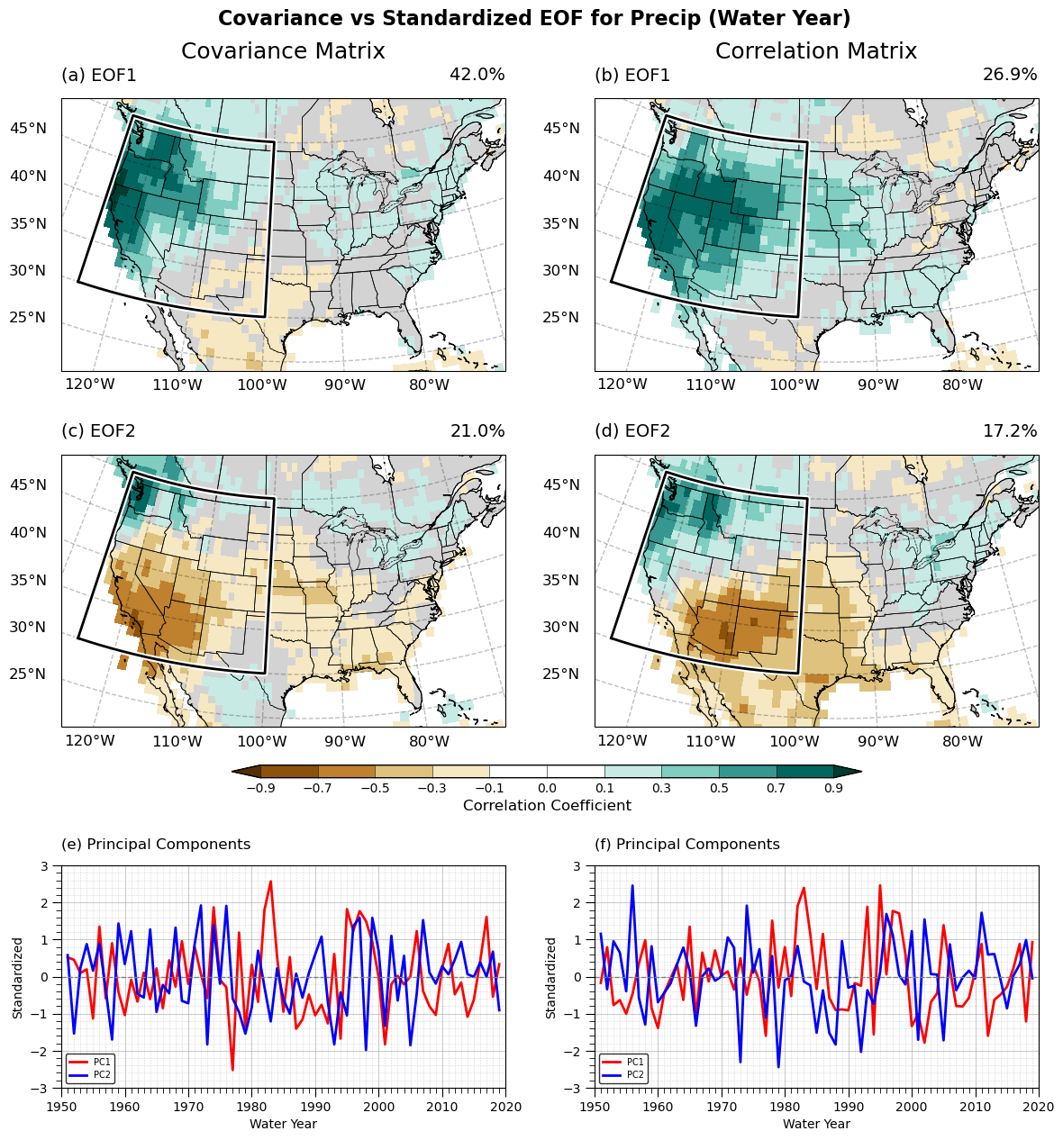
fig.suptitle("Covariance vs Standardized EOF for Precip (Water Year)", fontsize=16, fontweight="bold")
grid = plt.GridSpec(3, 2, height_ratios=[1.2, 1.0, 1.4], hspace=0.1)
# === Setup Global Settings ===
projection = ccrs.LambertConformal(central_longitude=-95.0, standard_parallels=(29.5, 45.5))
contour_levels = np.array([-0.9, -0.7, -0.5, -0.3, -0.1, 0, 0.1, 0.3, 0.5, 0.7, 0.9])
color_indices = [0, 1, 2, 3, 4, 'transparent', 'transparent', 6, 7, 8, 9, 10]
# Then manually define colors:
selected_colors = []
for idx in color_indices:
if idx == 'transparent':
selected_colors.append((0, 0, 0, 0)) # Transparent
else:
selected_colors.append(cmaps.CBR_drywet.colors[idx])
selected_cmap = ListedColormap(selected_colors, name="selected_CBR_drywet")
norm = BoundaryNorm(boundaries=contour_levels, ncolors=len(selected_colors), extend='both')
#color_indices = [0, 1, 2, 3, 4, 5, 5, 6, 7, 8, 9, 10]
#selected_colors = [cmaps.CBR_drywet.colors[i] for i in color_indices]
#selected_cmap = ListedColormap(selected_colors, name="selected_CBR_drywet")
#norm = BoundaryNorm(boundaries=contour_levels, ncolors=len(selected_colors), extend='both')
# === Define Axis Setup Function ===
def setup_axis(ax, ystr, yend, ymin=-3, ymax=3, y_major=1, y_minor=0.2):
ax.set_xlim(pd.to_datetime(f"{ystr}"), pd.to_datetime(f"{yend}"))
ax.xaxis.set_major_locator(mdates.YearLocator(10))
ax.xaxis.set_minor_locator(mdates.YearLocator(1))
ax.xaxis.set_major_formatter(mdates.DateFormatter("%Y"))
ax.set_ylim(ymin, ymax)
ax.yaxis.set_major_locator(MultipleLocator(y_major))
ax.yaxis.set_minor_locator(MultipleLocator(y_minor))
ax.grid(visible=True, which="major", linestyle="-", linewidth=0.7, alpha=0.7)
ax.grid(visible=True, which="minor", linestyle="--", linewidth=0.4, alpha=0.5)
ax.tick_params(axis="both", which="major", length=7)
ax.tick_params(axis="both", which="minor", length=4)
# === Define Overlay Time Series Plot Function ===
def plot_overlay_ts(ax, pc1, pc2, title, label1="PC1", label2="PC2", ystr=1950, yend=2020):
years_dt = pd.to_datetime(pc1["year"].values.astype(str))
ax.plot(years_dt, pc1, color="red", linewidth=2, label=label1)
ax.plot(years_dt, pc2, color="blue", linewidth=2, label=label2)
ax.axhline(0, color="gray", linestyle="--", linewidth=1)
setup_axis(ax, ystr, yend)
gvutil.set_titles_and_labels(ax, maintitle="", lefttitle=title, lefttitlefontsize=12,
xlabel="Water Year", ylabel="Standardized", labelfontsize=10)
ax.legend(loc="lower left", fontsize=7, frameon=True, edgecolor="black")
ax.set_box_aspect(0.5)
# Map axes
ax1 = fig.add_subplot(grid[0, 0], projection=projection)
ax2 = fig.add_subplot(grid[0, 1], projection=projection)
ax3 = fig.add_subplot(grid[1, 0], projection=projection)
ax4 = fig.add_subplot(grid[1, 1], projection=projection)
# Time series axes
ax5 = fig.add_subplot(grid[2, 0])
ax6 = fig.add_subplot(grid[2, 1])
# --- Plot Maps ---
setup_map(ax1, "Covariance Matrix", "(a) EOF1", pcs_cov.attrs['varianceFraction'][0], latlonEOF)
im1 = ax1.pcolormesh(cor1_cov["lon"], cor1_cov["lat"], cor1_cov, cmap=selected_cmap, norm=norm, shading="auto", transform=ccrs.PlateCarree())
draw_projected_box(ax1, latlonEOF)
setup_map(ax2, "Correlation Matrix", "(b) EOF1", pcs_std.attrs['varianceFraction'][0], latlonEOF)
im2 = ax2.pcolormesh(cor1_std["lon"], cor1_std["lat"], cor1_std, cmap=selected_cmap, norm=norm, shading="auto", transform=ccrs.PlateCarree())
draw_projected_box(ax2, latlonEOF)
setup_map(ax3, "", "(c) EOF2", pcs_cov.attrs['varianceFraction'][1], latlonEOF)
im3 = ax3.pcolormesh(cor2_cov["lon"], cor2_cov["lat"], cor2_cov, cmap=selected_cmap, norm=norm, shading="auto", transform=ccrs.PlateCarree())
draw_projected_box(ax3, latlonEOF)
setup_map(ax4, "", "(d) EOF2", pcs_std.attrs['varianceFraction'][1], latlonEOF)
im4 = ax4.pcolormesh(cor2_std["lon"], cor2_std["lat"], cor2_std, cmap=selected_cmap, norm=norm, shading="auto", transform=ccrs.PlateCarree())
draw_projected_box(ax4, latlonEOF)
# --- Plot Time Series ---
plot_overlay_ts(ax5, pc1_cov, pc2_cov, "(e) Principal Components")
plot_overlay_ts(ax6, pc1_std, pc2_std, "(f) Principal Components")
# --- Shared Colorbar between maps and time series ---
cbar_ax = fig.add_axes([0.26, 0.37, 0.5, 0.010]) # Adjust carefully between map and TS
cbar = plt.colorbar(im1, cax=cbar_ax, orientation="horizontal", spacing="uniform", extend='both',
ticks=contour_levels, drawedges=True)
cbar.set_label("Correlation Coefficient", fontsize=12)
cbar.ax.tick_params(length=0, labelsize=10)
cbar.outline.set_edgecolor("black")
cbar.outline.set_linewidth(1.0)
# --- Layout Adjustments ---
plt.subplots_adjust(top=0.94, bottom=0.05)
plt.savefig(fnFIG, dpi=300, bbox_inches="tight")
plt.show()