General Visualization

# --- Packages ---
## General Packages
import pandas as pd
import xarray as xr
import numpy as np
import os
import ipynbname
import cftime

## GeoCAT
import geocat.comp as gccomp
import geocat.viz as gv
import geocat.viz.util as gvutil

## Regridding and geopandas
#import xesmf as xe
#import geopandas as gpd

## Visualization
import cmaps  
import cartopy.crs as ccrs
import cartopy.feature as cfeature
import shapely.geometry as sgeom

## MatPlotLib
import matplotlib.pyplot as plt
import matplotlib.ticker as mticker
import matplotlib.patches as mpatches
import matplotlib.dates as mdates
import matplotlib.patheffects as pe

from matplotlib.colors import ListedColormap, BoundaryNorm
from matplotlib.ticker import MultipleLocator

## Unique Plots
import matplotlib.gridspec as gridspec

# NCL Fonts
plt.rcParams["font.family"] = "DejaVu Sans"
plt.rcParams["font.size"] = 12

def get_filename(default="figure"):
    """Return the base filename of the current script or notebook."""
    # Case 1: running from a .py file
    if "__file__" in globals():
        return os.path.splitext(os.path.basename(__file__))[0]
    # Case 2: running inside Jupyter Notebook
    try:
        import ipynbname
        nb_path = ipynbname.path()
        return os.path.splitext(os.path.basename(str(nb_path)))[0]
    except Exception:
        # Fallback
        return default

# --- Example usage ---
base = get_filename("template_eof_US")
fnFIG  = f"{base}.png"
fnEPS = f"{base}.eps"

print(f"Figure filename: {fnFIG}")

Figure filename: template_eof_US.png

# --- DATA ANALYSIS ---

# Replace this block
ystr, yend = 1950, 2020
years = np.arange(ystr, yend + 1)
values = np.random.randn(len(years))  # or use np.random.rand() for [0, 1] range
dat = xr.DataArray(values, coords={"year": years},
    dims=["year"], name="dummy data")
print(dat)

<xarray.DataArray 'dummy data' (year: 71)> Size: 568B
array([ 0.69932233, -0.6093763 ,  0.67189332,  1.97906076, -0.81673206,
        1.67922097,  0.30852525, -0.72564273, -0.6447174 , -0.8106967 ,
        0.92338843, -0.65660246, -0.0963152 ,  0.28801701,  1.1160102 ,
       -0.7460441 ,  0.68567217, -0.08745197, -0.2073813 ,  0.64519905,
       -0.11132989, -0.98549081, -1.2874477 ,  1.72442407,  0.61082668,
        0.58468168,  0.18478763,  0.00654854,  1.52252192, -0.06981891,
        1.65067853,  0.7542871 ,  0.01738674, -0.04042116,  1.40534851,
        0.61962906,  0.07324505,  0.02647415, -1.696394  ,  0.1893059 ,
       -0.08935942, -2.16892536,  1.69673889, -0.44076272, -1.11807339,
       -0.52963602,  0.51741634, -0.96915918,  0.19612623, -0.16686904,
       -2.03557351, -1.103211  ,  0.55669881, -0.46581984, -1.6025464 ,
        1.34173298, -0.25367901, -1.28358274, -0.42832301,  1.57902386,
        0.5630813 , -2.48908172, -0.46010296, -1.3882786 , -0.6416944 ,
       -0.56762194,  1.88920058,  1.87062293,  0.07954066,  1.41543906,
       -0.98329272])
Coordinates:
  * year     (year) int64 568B 1950 1951 1952 1953 1954 ... 2017 2018 2019 2020

# --- FIGURE PLOT ---
# Layout setting
fig, axes = plt.subplots(nrows=3, ncols=1, figsize=(8, 12))
col = cmaps.amwg  # Use the AMWG colormap

axes = axes.flatten()  # 🔑 Make it a 1D list of axes

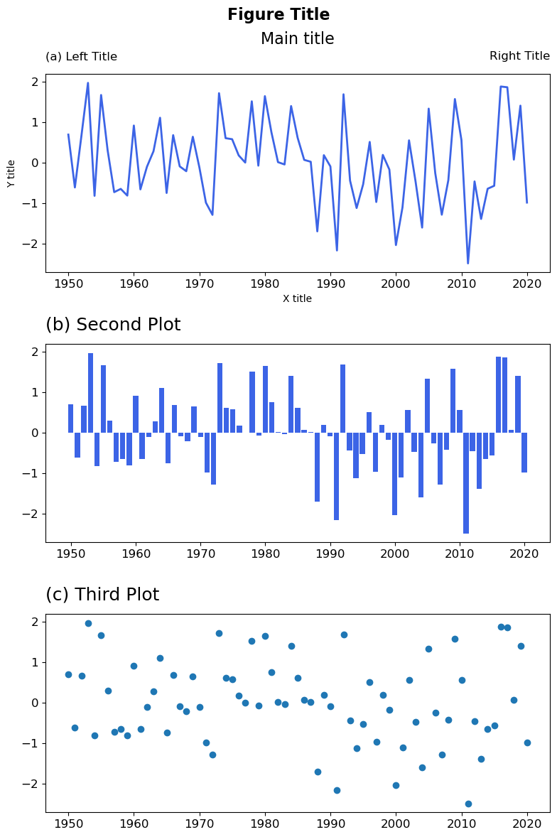
# --- Plot 1 ---
ip = 0
axes[ip].plot(dat.year, dat, label="Label", color=col.colors[4-2], linewidth=2)
gvutil.set_titles_and_labels(axes[ip],
    maintitle="Main title",
    lefttitle="(a) Left Title",
    righttitle="Right Title",
    ylabel="Y title",
    xlabel="X title",
    maintitlefontsize=14,  # Adjust main title font size
    lefttitlefontsize=12,  # Set left title font size
    righttitlefontsize=12,  # Set left title font size
    labelfontsize=10  # Set y-label font size
)

# --- Plot 2 ---
ip = 1
axes[ip].bar(dat.year, dat, label="Label", color=col.colors[4-2], linewidth=2)
gvutil.set_titles_and_labels(axes[ip],
    lefttitle="(b) Second Plot",
)

# --- Plot 3 ---
ip = 2
axes[ip].plot(dat.year, dat, marker="o", linestyle="None", markersize=6)
gvutil.set_titles_and_labels(axes[ip],
    lefttitle="(c) Third Plot",
)


# Apply the overall figure title
fig.suptitle("Figure Title", fontsize=16, fontweight="bold")

# --- OUTPUT ---
plt.tight_layout()
plt.savefig(fnFIG, dpi=300, bbox_inches="tight")
plt.show()